Chapter 2 Second break-out room
We will calculated four different beta diversities: Bray-Curtis, Jaccard, unweighted UniFrac and Weighted UniFrac and use Principal Coordinates Analysis (PCoA, = Multidimensional scaling, MDS). This is a method to explore and to visualize similarities or dissimilarities of data.
2.1 Calculate beta-diversities
set.seed(12345)
metadata <- as(sample_data(ps1), "data.frame")

ord <- ordinate(ps1, method = "PCoA", distance = "bray")
p <- plot_ordination(ps1, ord, color = "Feed",  label="Pen", shape= "PenNr")
p1 <- p + theme_bw()  + ggtitle("PCoA Bray Curtis")
p1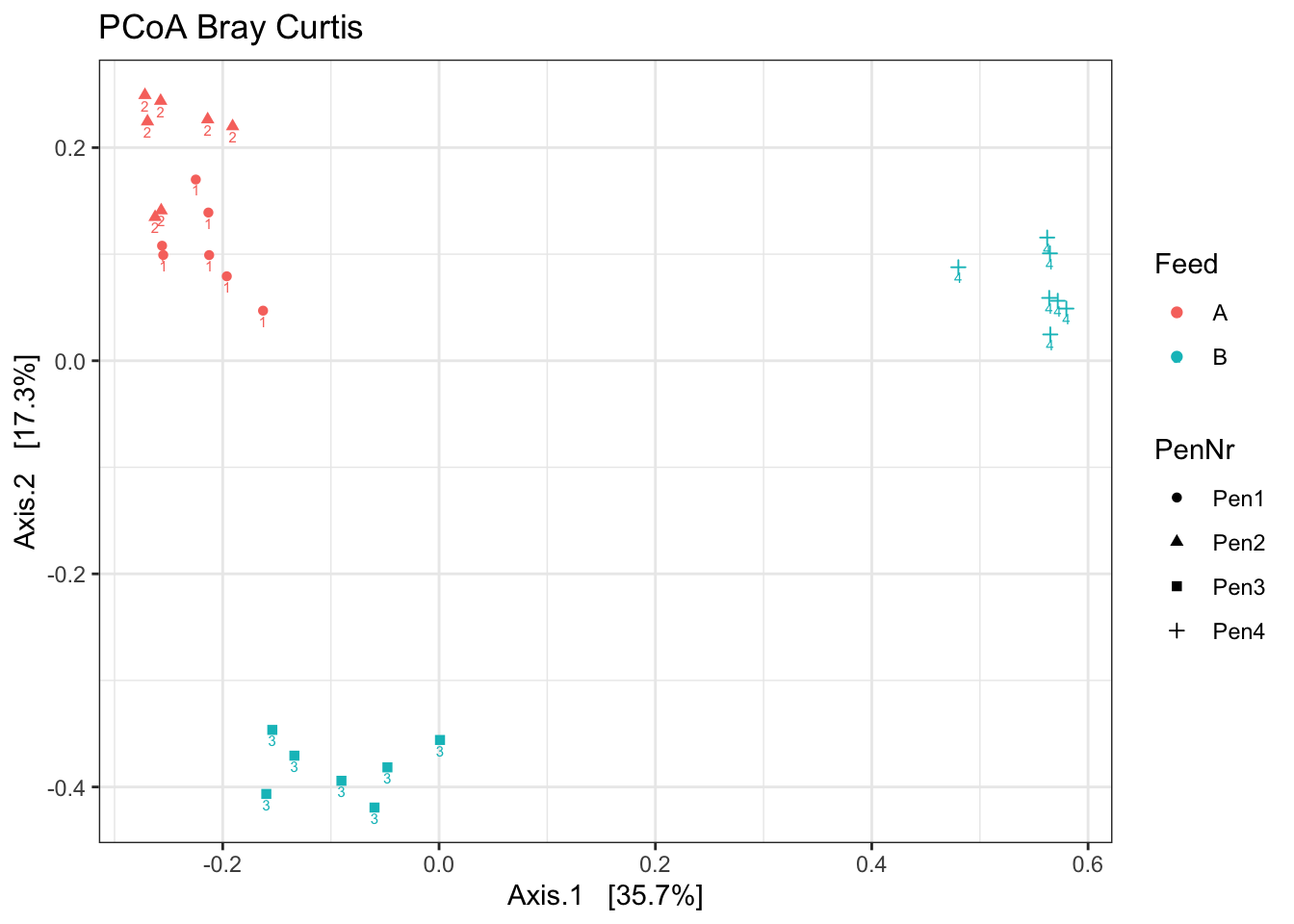
ord <- ordinate(ps1, method = "PCoA", distance = "jaccard", binary = TRUE) ##binary = TRUE!
p <- plot_ordination(ps1, ord, color = "Feed",   label="Pen", shape= "PenNr")
p1 <- p + theme_bw()  + ggtitle("PCoA Jaccard")
p1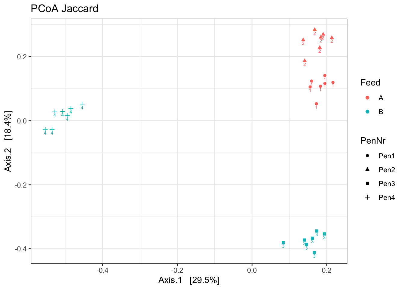
ord <- ordinate(ps1, method = "PCoA", distance = "wunifrac")
p <- plot_ordination(ps1, ord, color = "Feed",   label="Pen", shape= "PenNr")
p1 <- p + theme_bw()  + ggtitle("PCoA wunifrac")
p1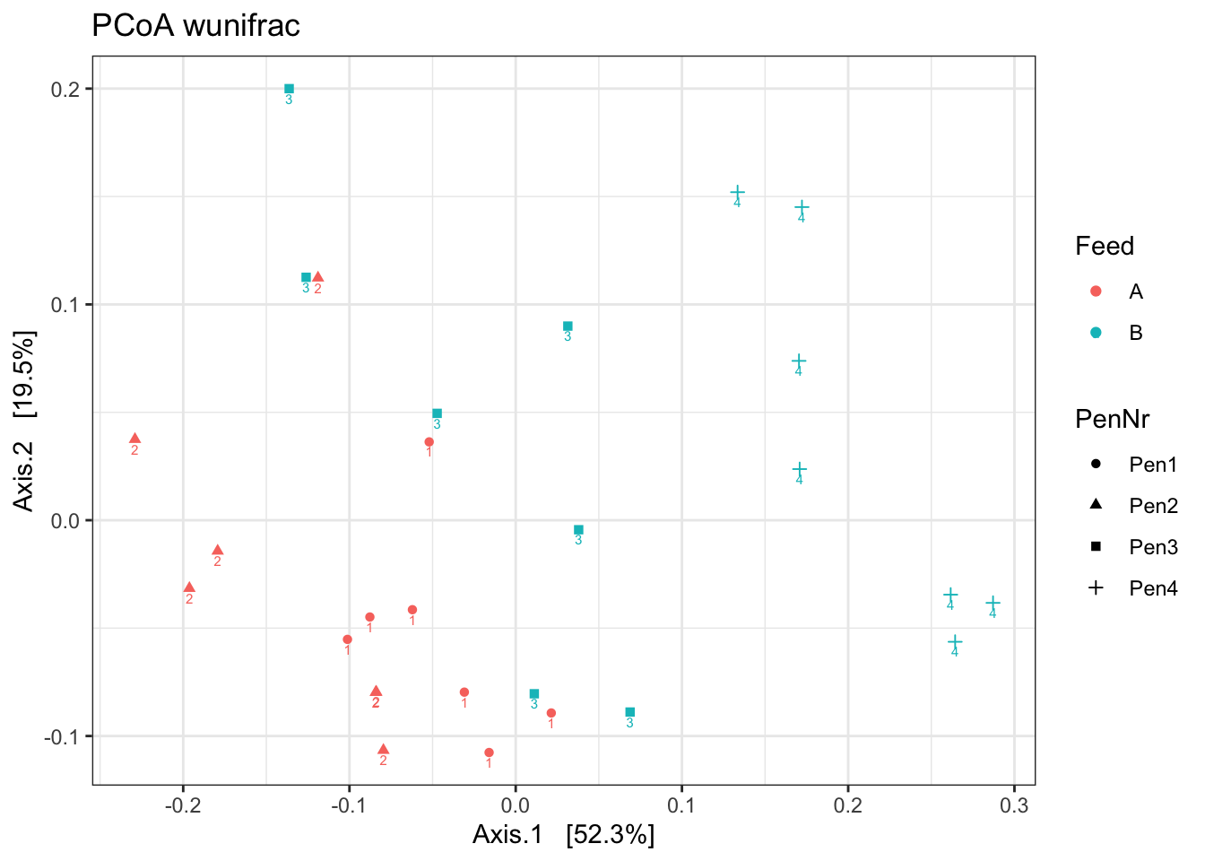
ord <- ordinate(ps1, method = "PCoA", distance = "unifrac")
p <- plot_ordination(ps1, ord, color = "Feed",  label="Pen", shape= "PenNr")
p1 <- p + theme_bw()  + ggtitle("PCoA unifrac")
p1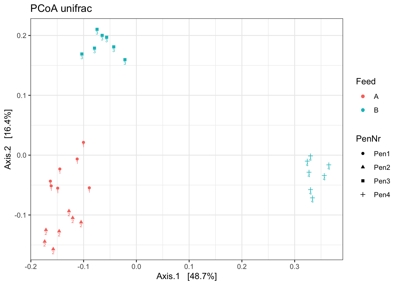
What stands out?
Which beta diversity would you use?
2.2 PERMANOVA
dist.b <- phyloseq::distance(ps1, method = "bray")
dist.j <- phyloseq::distance(ps1, method = "jaccard", binary = TRUE)
dist.uf <- phyloseq::distance(ps1, method = "unifrac")
dist.wuf <- phyloseq::distance(ps1, method = "wunifrac")


adonis(dist.b ~ Feed, data = metadata, perm=9999)
##
## Call:
## adonis(formula = dist.b ~ Feed, data = metadata, permutations = 9999)
##
## Permutation: free
## Number of permutations: 9999
##
## Terms added sequentially (first to last)
##
## Df SumsOfSqs MeanSqs F.Model R2 Pr(>F)
## Feed 1 2.2000 2.2000 9.1588 0.2605 1e-04 ***
## Residuals 26 6.2453 0.2402 0.7395
## Total 27 8.4453 1.0000
## ---
## Signif. codes: 0 '***' 0.001 '**' 0.01 '*' 0.05 '.' 0.1 ' ' 1ps.disper <- betadisper(dist.b, metadata$Feed)
permutest(ps.disper)##
## Permutation test for homogeneity of multivariate dispersions
## Permutation: free
## Number of permutations: 999
##
## Response: Distances
## Df Sum Sq Mean Sq F N.Perm Pr(>F)
## Groups 1 0.010126 0.0101263 2.3739 999 0.132
## Residuals 26 0.110907 0.0042656adonis(dist.j ~ Feed, data = metadata, perm=9999) ##
## Call:
## adonis(formula = dist.j ~ Feed, data = metadata, permutations = 9999)
##
## Permutation: free
## Number of permutations: 9999
##
## Terms added sequentially (first to last)
##
## Df SumsOfSqs MeanSqs F.Model R2 Pr(>F)
## Feed 1 1.8183 1.81828 7.3404 0.22017 1e-04 ***
## Residuals 26 6.4404 0.24771 0.77983
## Total 27 8.2587 1.00000
## ---
## Signif. codes: 0 '***' 0.001 '**' 0.01 '*' 0.05 '.' 0.1 ' ' 1ps.disper <- betadisper(dist.j, metadata$Feed)
permutest(ps.disper)##
## Permutation test for homogeneity of multivariate dispersions
## Permutation: free
## Number of permutations: 999
##
## Response: Distances
## Df Sum Sq Mean Sq F N.Perm Pr(>F)
## Groups 1 0.047419 0.047419 17.286 999 0.001 ***
## Residuals 26 0.071322 0.002743
## ---
## Signif. codes: 0 '***' 0.001 '**' 0.01 '*' 0.05 '.' 0.1 ' ' 1adonis(dist.uf ~ Feed, data = metadata, perm=9999) ##
## Call:
## adonis(formula = dist.uf ~ Feed, data = metadata, permutations = 9999)
##
## Permutation: free
## Number of permutations: 9999
##
## Terms added sequentially (first to last)
##
## Df SumsOfSqs MeanSqs F.Model R2 Pr(>F)
## Feed 1 0.70667 0.70667 11.734 0.31096 1e-04 ***
## Residuals 26 1.56590 0.06023 0.68904
## Total 27 2.27257 1.00000
## ---
## Signif. codes: 0 '***' 0.001 '**' 0.01 '*' 0.05 '.' 0.1 ' ' 1ps.disper <- betadisper(dist.uf, metadata$Feed)
permutest(ps.disper)##
## Permutation test for homogeneity of multivariate dispersions
## Permutation: free
## Number of permutations: 999
##
## Response: Distances
## Df Sum Sq Mean Sq F N.Perm Pr(>F)
## Groups 1 0.025001 0.0250014 38.108 999 0.001 ***
## Residuals 26 0.017058 0.0006561
## ---
## Signif. codes: 0 '***' 0.001 '**' 0.01 '*' 0.05 '.' 0.1 ' ' 1adonis(dist.wuf ~ Feed, data = metadata, perm=9999) ##
## Call:
## adonis(formula = dist.wuf ~ Feed, data = metadata, permutations = 9999)
##
## Permutation: free
## Number of permutations: 9999
##
## Terms added sequentially (first to last)
##
## Df SumsOfSqs MeanSqs F.Model R2 Pr(>F)
## Feed 1 0.31792 0.31792 11.132 0.2998 1e-04 ***
## Residuals 26 0.74253 0.02856 0.7002
## Total 27 1.06045 1.0000
## ---
## Signif. codes: 0 '***' 0.001 '**' 0.01 '*' 0.05 '.' 0.1 ' ' 1ps.disper <- betadisper(dist.wuf, metadata$Feed)
permutest(ps.disper)##
## Permutation test for homogeneity of multivariate dispersions
## Permutation: free
## Number of permutations: 999
##
## Response: Distances
## Df Sum Sq Mean Sq F N.Perm Pr(>F)
## Groups 1 0.018811 0.0188112 8.6956 999 0.009 **
## Residuals 26 0.056246 0.0021633
## ---
## Signif. codes: 0 '***' 0.001 '**' 0.01 '*' 0.05 '.' 0.1 ' ' 1Which beta diversity explained most of the variation with the factor feed?
Additional reading Gloor et al., 2017: Microbiome Datasets Are Compositional: And This Is Not Optional Paliy and Shankar, 2016: Application of multivariate statistical techniques in microbial ecology